Running BayesEoR
scripts/run-analysis.py provides an example driver script for running BayesEoR. This file contains all of the necessary steps to set up the bayeseor.posterior.PowerSpectrumPosteriorProbability class and to run MultiNest and obtain power spectrum posteriors.
There are currently two steps involved in a BayesEoR analysis
Build the required matrices (CPUs only, no GPUs or MPI required)
Run the power spectrum analysis (double precision GPUs recommended)
Below, we provide some useful information about the required Inputs and Analysis Steps. For additional help with running BayesEoR and setting analysis parameters, please see Setting Parameters. More information on running BayesEoR can also be found in Test Datasets.
Inputs
BayesEoR requires the following as inputs to run a power spectrum analysis:
Analysis parameters
Visibilities
Instrument model
More information about each of these components can be found below.
Analysis Parameters
BayesEoR is configured via a set of analysis parameters which can be set via a configuration yaml file (recommended) or the command line. The provided configuration file (test_data/eor/config.yaml) provides an example of the minimum sufficient set of analysis parameters for a power spectrum analysis when using a pyuvdata-compatible file as input (more on this in the section below on Visibilities). Please see Setting Parameters for the contents of this file and bayeseor.params.BayesEoRParser for a description of each of the user-definable analysis parameters. The full list of parameters can also be displayed by running
python run-analysis.py --help
Some of the analysis parameters have quite obvious values. For example, nf and nt are simply the number of frequencies and times in the data being analyzed, respectively. Other parameters require a little more care. The parameters nu (the number of sampled Fourier modes along the u axis of the model uv plane) and fov_ra_eor (the field of view of the sky model along the right ascension axis) must be chosen more carefully. In addition to the field of view of the sky model, fov_ra_eor also determines the spacing between adjacent modes along the u axis of the model uv plane. The value of nu must therefore be chosen to fully encompass the u coordinates sampled by the baselines in the input data. The beam must also be taken into account when choosing nu for a given fov_ra_eor as the beam effects the extent of the uv plane sampled by each baseline. The same arguments apply when choosing nv and fov_dec_eor as these quantities correspond to the v axis of the model uv plane and the declination axis of the sky model, respectively. Please see section 2.3 of Burba et al. 2023a for a more detailed discussion on choosing model parameters.
Visibilities
The input data are visibilities and are specified via the data_path (--data-path) argument in the configuration file (on the command line). They can be read in as a pyuvdata- (recommended) or numpy-compatible file. The required analysis parameters differ for each input and are described below.
pyuvdata-Compatible File
This is the recommended format for input data
Visibilities can be read via pyuvdata in .uvh5, .uvfits, or .ms format (measurement set functionality in pyuvdata requires an optional dependency of casacore). This is the recommended method for specifying input visibilities as no data preprocessing step is required (more on this in the subsection below). The data can be downselected via a suite of configuration file (command line) arguments, a subset of which is presented here:
ant_str(--ant-str): antenna downselect stringbl_cutoff(--bl-cutoff): maximum baseline length, \(b=\sqrt{u^2 + v^2}\), in meterspol(--pol): polarization string, e.g. ‘xx’, ‘yy’, ‘pI’form_pI(--form-pI): form pseudo-Stokes I visibilities from XX and YY visibilities via pI = N * (XX + YY) where N is a user-specified normalization set viapI_norm(--pI-norm) which defaults to 1.0--redundant-avg(redundant_avg): redundantly average visibilitiesfreq_min(--freq-min): minimum frequency in hertznf(--nf): number of frequenciesjd_min(--jd-min): minimum Julian datent(--nt): number of times
For a complete list of parameters, please see Parameters. For more information on the ant_str and pol arguments, please see the pyuvdata.UVData.select documentation. For more information on the redundant averaging, please see the pyuvdata.UVData.compress_by_redundancy documentation.
At runtime, a one-dimensional vector of visibilities, and the corresponding instrument model (see Instrument Model below), is formed based on the contents of the pyuvdata-compatible file and the user-specified analysis parameters. This visibility vector can be saved to disk for later use by setting the save_vis kwarg to True when calling bayeseor.setup.run_setup (or by setting save_vis: True in the configuration file (--save-vis on the command line) when using the driver script). The location in which the visibility vector is saved can be specified by the save_dir kwarg in bayeseor.setup.run_setup. By default, when using the driver script, the visibility vector will be saved to the output directory containing the sampler outputs if save_vis is True.
numpy-Compatible File
Alternatively, visibilities can be read via numpy in the form of a preprocessed, one-dimensional vector. In this case, the input dataset is expected to be a numpy-compatible dictionary with a complex, one-dimensional vector of visibilities with shape (Nvis,) accessible via the "data" key. Here, Nvis = Nbls * Ntimes * Nfreqs is the total number of visibilities and Nbls, Ntimes, and Nfreqs are the number of baselines, times, and frequencies in the data. The ordering of the baselines in this one-dimensional vector is arbitrary. However, this order must align with the ordering of the baselines in the instrument model (more on this below in Instrument Model).
If passing a numpy-compatible file as input, the following analysis parameters are required as configuration file (command line) arguments:
Frequency parameters:
nf(--nf): number of frequenciesdf(--df): frequency channel width in hertzfreq_min(--freq-min): minimum frequency in hertz ORfreq_center(--freq-center): central frequency in hertz
Time parameters:
nt(--nt): number of timesdt(--dt): integration time in secondsjd_min(--jd-min): minimum Julian date ORjd_center(--jd-center): central Julian date
Instrument model parameters:
inst_model(--inst-model): path to the directory containing the instrument model (see Instrument Model below)
This numpy-compatible dictionary can be generated via bayeseor.setup.run_setup with save_vis set to True (and save_dir specifying the output location for the dictionary). This is an optional preprocessing step and is not required as the data vector can be generated at runtime if a pyuvdata-compatible file is passed via data_path. However, preprocessing the data vector and saving it to disk can be potentially beneficial if the pyuvdata-compatible file you are reading from is large.
Instrument Model
The instrument model is comprised of the following components:
“uv sampling”: the (u, v, w) coordinates sampled by each baseline with shape (Ntimes, Nbls, 3)
Redundancy model: the number of redundantly-averaged baselines per (u, v, w) coordinate in the uv sampling with shape (Ntimes, Nbls, 1)
Primary beam model: either a path to a UVBeam-compatible file or a string specifying an analytic beam profile (more on this below)
Phasor vector (optional): an array which phases the visibilities as a function of time with shape (Nvis,)
The inst_model (--inst-model) argument in the configuration file (on the command line) specifies the directory containing the uv sampling, redundancy, and, optionally, the phasor vector. Just like the visibility vector, these quantities should be stored in numpy-compatible dictionaries, one for each component, where the data are accessed via the "data" key. By default, BayesEoR looks for the following file names in the instrument model directory for these three components: uvw_model.npy (uv sampling), redundancy_model.npy (redundancy), phasor_vector.npy (optional phasor vector). The primary beam model is set via a separate set of arguments. The most important primary beam model parameter is beam_type (--beam-type) which can contain a path to a pyuvdata.UVBeam-compatible file or a string specifying an analytic beam type (e.g. "uniform", "gaussian", "airy"). Each analytic beam type has its own set of required parameters. Please see Setting Parameters or bayeseor.model.healpix.Healpix for details on supported analytic beam types and their associated parameters.
Quantities 1-3 are required in every analysis. Quantity 4, the phasor vector, is optional and is only used if modelling phased visibilities. In our experience, we have found that we recover more accurate model visibilities when the data and model are unphased. For this reason, we suggest modelling unphased visibilities and excluding the phasor vector from the instrument model.
The uv sampling, redundancy model, and optional phasor vector are all generated by bayeseor.setup.run_setup when the input data is a pyuvdata-compatible file. These arrays can be saved to disk as numpy-compatible dictionaries for later use by setting the save_model kwarg to True in bayeseor.setup.run_setup (or using --save-model on the command line or setting save_model: True in the configuration yaml). bayeseor.setup.run_setup also write the antenna pair tuples, (ant1, ant2), to disk when generating the instrument model (antpairs.npy), but this is not a required input for the instrument model. The location in which these dictionaries are saved can be specified by the save_dir kwarg in bayeseor.setup.run_setup. By default, when using the driver script, these arrays will be saved to the output directory containing the sampler outputs if save_model is True.
Analysis Steps
Building the Matrix Stack
If using a configuration file (recommended), the driver script can be run to build the matrices via
python scripts/run-analysis.py --config /path/to/config.yaml --cpu
Note that with jsonargparse, command line arguments that come after the --config flag overwrite the value of the argument in the configuration file. In the example above, the --cpu flag placed after the --config flag will force the code to use CPUs only.
BayesEoR automatically creates a directory in which to store the matrix stack if one does not already exist. The name of the matrix stack directory is set automatically based on the chosen analysis parameters. The prefix for this matrix stack directory can be set via the array_dir_prefix (--array-dir-prefix) argument in the configuration yaml (on the command line). The matrix stack is saved in a subdirectory within array_dir_prefix. The default matrix stack prefix is ./matrices/.
Warning
The matrix stack build methods do not support MPI. MPI is only supported during power spectrum analysis. If the matrix stack is built using multiple MPI processes, all processes except rank 0 will raise an error and exit. The matrix stack will continue building on rank 0.
Tip
Using multiple CPUs will speed up the matrix construction as, for dense-dense matrix operations, we can take advantage of numpy’s built-in threading.
Running the Power Spectrum Analysis
Once the matrices are built, you can run the power spectrum analysis (for which we highly recommend using double precision GPUs) via
python scripts/run-analysis.py --config /path/to/config.yaml --gpu --run
The --run flag (or run: True in the configuration yaml) is required to run the power spectrum analysis. Otherwise, only the bayeseor.posterior.PowerSpectrumPosteriorProbability class will be instantiated (which can be useful for testing in an interactive python environment). As above, the trailing --gpu flag will force the code to use GPUs. When passing --gpu (or setting use_gpu: True in the configuration yaml), the power spectrum analysis will only run if at least one GPU is found and the GPU initialization is successful.
Outputs
The location for the outputs of a BayesEoR analysis can be set via the output_dir argument in the configuration yaml or the --output-dir flag on the command line. The output files from BayesEoR will be placed in a subdirectory of output_dir, which we refer to internally as file_root, and the name of file_root is set automatically based on the chosen analysis parameters. The default output directory prefix is ./chains/.
In the sampler output directory, i.e. Path(output_dir) / file_root, BayesEoR outputs a few key files:
version.txt: simple text file with thebayeseorversion used in the analysisargs.json: JSON file containing all of the configuration / command line arguments used in the analysisk-vals*.txt: \(k\) bin information filesk-vals.txt: mean of each \(k\) bink-vals-bins.txt: bin edges of each \(k\) bink-vals-nsamples.txt: number of \(\vec{k}\) in each \(k\) bin
data-*: These files contain the outputs of the sampler, the most important beingdata-.txt. This file contains the sampler output and has the power spectrum amplitude samples for each iteration. For MultiNest outputs, this file has \(N_k\) + 2 columns where \(N_k\) is the number of spherically-averaged \(k\) bins. The columns of interest in this file are the columns with index 0 and >= 2. The 0th column contains the joint posterior probability value per iteration. The columns with index >= 2 contain the power spectrum amplitude samples for each \(k\) bin.
For convenience, we have provided a class to aid in analyzing these outputs. For more information on this class, please see Analyzing BayesEoR Outputs.
Analyzing BayesEoR Outputs
We have provided a basic class for analyzing the outputs of BayesEoR. The minimum requirement to instantiate the class is a list of directory names containing the BayesEoR output directories. There are also several kwargs you can set to calculate various quantities, compare the results with an expected power spectrum, and/or modify the attributes of the created plots. Please see bayeseor.analyze.analyze.DataContainer for more information.
As an example, let us consider the case of the outputs of an analysis using the provided EoR-only test data (see EoR Only for more details).
from bayeseor.analyze import DataContainer

dir_prefix = "./chains/"
dirnames = ["MN-15-15-38-0-2.63-2.82-6.2E-03-lp-dPS-v1/"]
expected_ps = 214777.66068216303  # mK^2 Mpc^3

data = DataContainer(
    dirnames,
    dir_prefix=dir_prefix,
    expected_ps=expected_ps,
    labels=["EoR Only"]
)
fig = data.plot_power_spectra_and_posteriors(
    suptitle="Test Data Analysis",
    plot_fracdiff=True,
    cred_interval=95
)
In this example, we’ve assumed the default output location ./chains/ and that the subdirectory containing the sampler outputs is MN-15-15-38-0-2.63-2.82-6.2E-03-lp-dPS-v1/.
Tip
If you wish to compare multiple analyses within the same directory, i.e. you have multiple subdirectories containing output files in ./chains/, you can add more entries to the dirnames kwarg e.g.
dirnames = ['MN-15-15-38-0-2.63-2.82-6.2E-03-lp-dPS-v1',
            'MN-15-15-38-0-2.63-2.82-6.2E-03-lp-dPS-v2',
            'MN-15-15-38-0-2.63-2.82-6.2E-03-lp-dPS-v3']
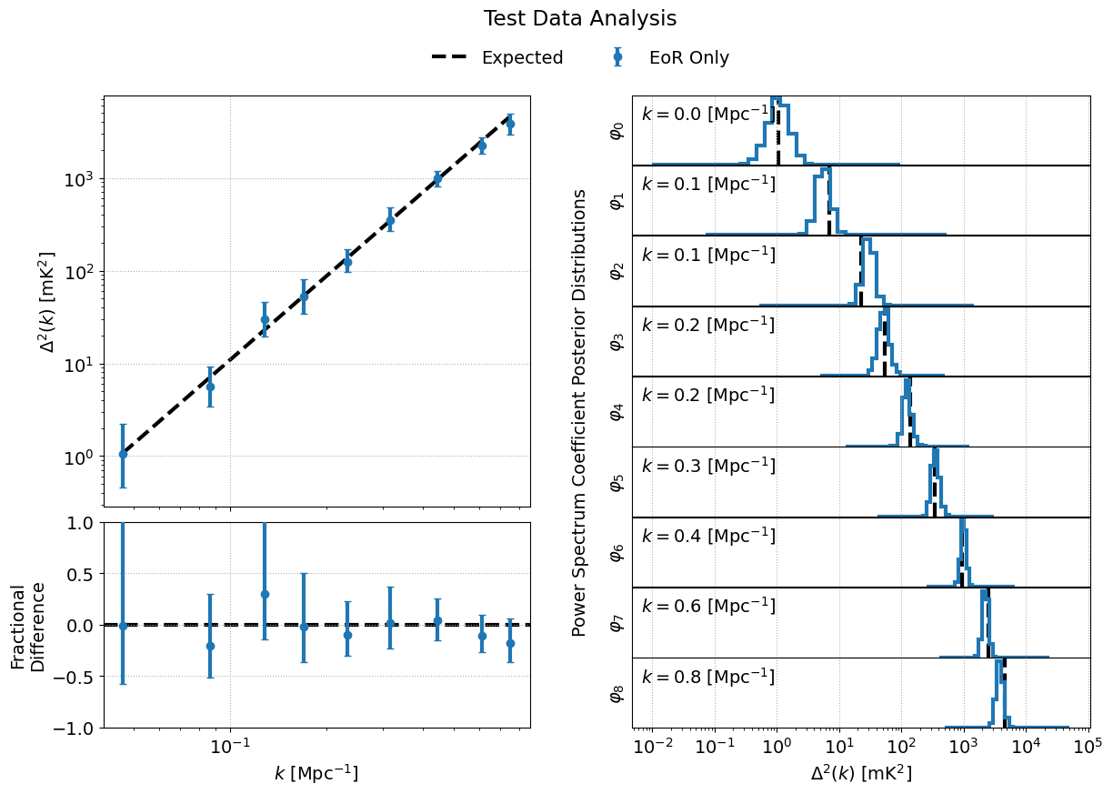
The variable expected_ps in the example above has been set specifically for the test dataset. The mock EoR signal in the test dataset has a flat power spectrum, \(P(k)\) (more info in the section above on the Test Datasets). We thus only need to specify a floating point number for the expected \(P(k)\). The class will internally convert this \(P(k)\) into the dimensionless power spectrum, \(\Delta^2(k)\), or vice versa, based on the combination of the ps_kind kwarg ('ps' for power spectrum or 'dmps' for the dimensionless power spectrum) and the expected_ps or expected_dmps kwargs. The default value of ps_kind is 'dmps', but we’ve passed the class the expected_ps kwarg corresponding to the power spectrum. The class will thus automatically convert this floating point \(P(k)\) into the corresponding \(\Delta^2(k)\) using the \(k\) bins files in each output directory.
The DataContainer class also provides a few plotting functions. In the example above, we’re using the plot_power_spectra_and_posteriors function which creates a summary plot containing a subplot for the power spectrum estimates, an optional difference (plot_diff=True) or fractional difference (plot_fracdiff=True) subplot if providing a known input power spectrum (via expected_ps or expected_dmps), and a subplot for the posterior of each \(k\) bin. The above code snippet will produce the following output if the analysis has been run correctly: