Test Datasets

The BayesEoR repository provides a set of test data and yaml configuration files for two simulated datasets: EoR only (test_data/eor/) and EoR + foregrounds (test_data/eor_fgs/). Both datasets share some common components described in the table below, Common simulation parameters. For more details on the simulated test data, please see Section 3 of Burba et al. 2023a.

Common simulation parameters
Parameter	Value
Minimum frequency	158.30 MHz
Frequency channel width	237.62 kHz
Number of frequencies	38
Minimum time (JD)	2458098.30
Integration time	11 s
Number of times	34
Beam type	Gaussian
Beam FWHM	9.3 deg
Number of baselines	15
Maximum baseline length	38.63 m

Instructions on using each test dataset are described below.

EoR Only

The EoR-only test data, test_data/eor/eor.uvh5, contain simulated visibilities of a mock EoR signal drawn as a Gaussian-random field with a flat power spectrum

\[P(k) = 214777.66068216303\ \rm{mK}^2\,\rm{Mpc}^3\]

BayesEoR outputs the dimensionless power spectrum, \(\Delta^2(k)\), which can be obtained from \(P(k)\) via

\[\Delta^2(k) = \frac{k^3}{2\pi^2}\,P(k)\]

The \(k\) bin values required to obtain the dimensionless power spectrum are written to disk automatically by BayesEoR in the same directory as the sampler outputs (please see Outputs or Analyzing BayesEoR Outputs for more information).

Analysis Parameters

A yaml configuration file has been provided which can be used to run the EoR-only test data analysis, test_data/eor/config.yaml:

# data_path can point to either a pyuvdata-compatible file (recommended) or
# a preprocessed numpy-compatible file generated via `bayeseor.setup.run_setup`
data_path: test_data/eor/eor.uvh5

# EoR model params
# Number of pixels along the u-axis of the model uv-plane
nu: 15
# nv can be set independently, but if None (default), nv will be set to nu
# nv: 15
# FoV of the image-space model in degrees along right ascension
fov_ra_eor: 12.9080728652
# The FoV of the declination axis of the image-space model, fov_dec_eor, can
# be set independently, buf it None (default), fov_dec_eor will be set to
# fov_ra_eor.
# fov_dec_eor: 12.9080728652
# Use a rectangular FoV for the image-space model.  Please note that using
# a rectangular FoV is not recommended (please see BayesEoR issue #11) and we
# recommend leaving simple_za_filter set to True (default).  For this
# particular test dataset, a rectangular FoV is okay.
simple_za_filter: False
# HEALPix nside parameter for the image-space model
nside: 128

# Noise model params
# The input data are noise free, so we need to simulate and add noise to the
# data vector.  sigma sets the standard deviation of the mean-zero Gaussian
# distribution from which the noise is drawn.  The amplitude has been chosen
# such that, in the visibility domain, the signal-to-noise ratio of the
# EoR-only visibility component to the noise component is 0.5.
sigma: 0.00615864342588761

# Instrument model params
# Telescope latitude [degrees], longitude [degrees], and altitude [meters]
telescope_latlonalt: [-30.72152777777791, 21.428305555555557, 1073.0000000093132]
# Beam type str as one of: uniform, gaussian, airy, gausscosine, or taperairy
beam_type: gaussian
# Full width at half maximum of the Gaussian beam
fwhm_deg: 9.306821090681533

# Prior params
# Prior [min, max] for each k bin in logarithmic units.  These priors have
# been chosen to be the true dimensionless power spectrum of the EoR-only
# visibilities plus or minus two orders of magnitude.
priors: [[-2.0, 2.0], [-1.2, 2.8], [-0.7, 3.3], [0.7, 2.7], [1.1, 3.1],
         [1.5, 3.5], [2.0, 4.0], [2.4, 4.4], [2.7, 4.7]]
# If you wish to set priors in linear units, you can do by setting log_priors
# to False and changing the prior min/max values above to linear units.
# log_priors: False

This yaml contains the minimum sufficient set of parameters to run an EoR only analysis. The input data in this case are visibilities in a pyuvdata-compatible file (test_data/eor/eor.uvh5). The frequency-axis parameters, freq_min (--freq-min), nf (--nf), and df (-df), and time-axis parameters, jd_min (--jd-min), nt (--nt), and dt (--dt), will all be extracted automatically from the input pyuvdata-compatible file, so they need not be explicitly specified in the configuration yaml. Because we are analyzing a pyuvdata-compatible file, there is also no need to specify an instrument model directory, inst_model (--inst-model). The instrument model will be generated at runtime using the baselines in test_data/eor/eor.uvh5.

Warning

The provided test data are simulated from a rectangular patch of sky with an arc length of 12.9 deg on each side. In the provided configuration yaml, we thus set simple_za_filter = False to use a rectangular FoV in the BayesEoR image-space model. In general, we discourage using a rectangular FoV in the image-space model (please see BayesEoR issue #11 for more details). In this particular case, the rectangular FoV is not an issue. When analyzing other datasets, we highly recommend setting simple_za_filter = True, its default value, to avoid any issues with rectangular FoV pixel selections. Please see Section 3 of Burba et al. 2023a for more details.

Build the Matrix Stack

To build the matrices (which will require ~17 GB of RAM and ~12 GB of disk space) using the provided example configuration yaml and test data, first navigate to the root directory of the BayesEoR repository. Then, run the following command

python scripts/run-analysis.py --config test_data/eor/config.yaml --cpu

The matrices will be stored in matrices/ in the current working directory.

Tip

If you wish to change the location in which the matrices are stored, specify the array_dir_prefix (--array-dir-prefix) argument in the configuration yaml (on the command line). Please see Setting Parameters for more details.

Run the Power Spectrum Analysis

Once the matrices are built, you can run the power spectrum analysis (which will require ~12 GB of RAM) via

python scripts/run-analysis.py --config test_data/eor/config.yaml --gpu --run

The sampler outputs will be stored in chains/MN-15-15-38-0-2.63-2.82-6.2E-03-lp-dPS-v1/.

Tip

If you wish to change the location in which the sampler outputs are stored, specify the output_dir (--output-dir) argument in the configuration yaml (on the command line). Please see Setting Parameters for more details.

Analyze the Outputs

We can use the bayeseor.analyze.analyze.DataContainer class to quickly analyze the outputs of the power spectrum analysis via

from bayeseor.analyze import DataContainer

dir_prefix = "./chains/"
dirnames = ["MN-15-15-38-0-2.63-2.82-6.2E-03-lp-dPS-v1/"]
expected_ps = 214777.66068216303  # mK^2 Mpc^3

data = DataContainer(
    dirnames,
    dir_prefix=dir_prefix,
    expected_ps=expected_ps,
    labels=["EoR Only"]
)
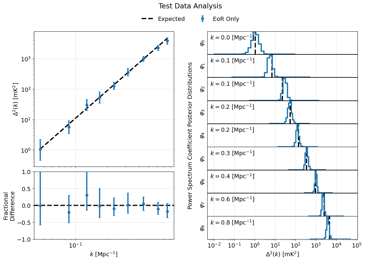
fig = data.plot_power_spectra_and_posteriors(
    suptitle="Test Data Analysis",
    plot_fracdiff=True,
    cred_interval=95
)

Attention

If you changed the location in which the sampler outputs are stored, you will need to update dir_prefix in the above code block to point to your specified output directory.

Tip

The bayeseor.analyze.analyze.DataContainer class calculates credibility intervals via the cred_intervals kwarg. You can specify any credibility intervals of interest as an e.g. list of percentages. By default, the 68% and 95% credibility intervals are calculated for each \(k\) bin. You can choose which credibility interval to plot as the uncertainty on each \(k\) bin in bayeseor.analyze.analyze.DataContainer.plot_power_spectra_and_posteriors() via the cred_interval kwarg.

This should produce the following figure if the analysis has been run correctly:

EoR and Foregrounds

The EoR + foregrounds test data, test_data/eor_fgs/eor_and_fgs.uvh5, contain simulated visibilities of the aforementioned mock EoR signal (EoR Only) plus diffuse and point source foregrounds. The diffuse component is the 2016 Global Sky Model (GSM) from Zheng et al. 2016 generated via PyGDSM. The point source component is a modified version of the GaLactic and Extragalactic All-sky MWA Survey (GLEAM) from Wayth et al. 2015. Please see section 3.2.2 of Burba et al. 2023a for the details of the modifications made to the GLEAM catalog.

Analysis Parameters

A yaml configuration file has been provided which can be used to run the EoR + foregrounds test data analysis, test_data/eor_fgs/config.yaml:

# data_path can point to either a pyuvdata-compatible file (recommended) or
# a preprocessed numpy-compatible file generated via `bayeseor.setup.run_setup`
data_path: test_data/eor_fgs/eor_and_fgs.uvh5

# EoR model params
# Number of pixels along the u-axis of the model uv-plane
nu: 15
# nv can be set independently, but if None (default), nv will be set to nu
# nv: 15
# FoV (diameter) of the image-space model in degrees along right ascension
fov_ra_eor: 12.9080728652
# The FoV of the declination axis of the image-space model, fov_dec_eor, can
# be set independently, buf it None (default), fov_dec_eor will be set to
# fov_ra_eor.
# fov_dec_eor: 12.9080728652
# Use a rectangular FoV for the image-space model.  Please note that using
# a rectangular FoV is not recommended (please see BayesEoR issue #11) and we
# recommend leaving simple_za_filter set to True (default).  For this
# particular test dataset, a rectangular FoV is okay.
simple_za_filter: False
# HEALPix nside parameter for the image-space model
nside: 128

# Foreground model params
# By default, the foreground model uv-plane will be built using nu and nv
# from the EoR model.  If you wish to specify a different nu or nv for the
# foreground model, you can do so via the nu_fg and nv_fg arguments below.
# If nv_fg is None (default), nv_fg will be set to nu_fg.
# nu_fg: 15
# nv_fg: 15
# The FoV parameters for the foreground model can also be set indepdently.
# If they are None (default), they will default to the corresponding EoR
# FoV parameters, i.e. fov_ra_fg = fov_ra_eor and fov_dec_fg = fov_dec_eor.
# fov_ra_fg: 12.9080728652
# fov_dec_fg: 12.9080728652
# Number of Large Spectral Scale Model (LSSM) basis vectors.  If beta is set
# to None, these basis vectors will be polynomials, e.g. for nq=2 the basis
# vectors would be freq and freq^2.  Note that the monopole eta=0 term is
# always modelled even if nq=0, thus there are nq+1 basis vectors in the LSSM.
# If beta is not None, as below, then the polynomial basis vectors are
# replaced with power laws where the entries in beta determine the _brightness
# temperature_ spectral indices.
nq: 2
# LSSM power law brightness temperature spectral indices
beta: [2.63, 2.82]
# Fit for a (u, v) = (0, 0) coefficient in the model uv-plane for each eta
fit_for_monopole: True

# Noise model params
# The input data are noise free, so we need to simulate and add noise to the
# data vector.  sigma sets the standard deviation of the mean-zero Gaussian
# distribution from which the noise is drawn.  The amplitude has been chosen
# such that, in the visibility domain, the signal-to-noise ratio of the
# EoR-only visibility component to the noise component is 0.5.
sigma: 0.00615864342588761

# Instrument model params
# Telescope latitude [degrees], longitude [degrees], and altitude [meters]
telescope_latlonalt: [-30.72152777777791, 21.428305555555557, 1073.0000000093132]
# Beam type str as one of: uniform, gaussian, airy, gausscosine, or taperairy
beam_type: gaussian
# Full width at half maximum of the Gaussian beam
fwhm_deg: 9.306821090681533

# Prior params
# Prior [min, max] for each k bin in logarithmic units.  These priors have
# been chosen to be the true dimensionless power spectrum of the EoR-only
# visibilities plus or minus two orders of magnitude.
priors: [[-2.0, 2.0], [-1.2, 2.8], [-0.7, 3.3], [0.7, 2.7], [1.1, 3.1],
         [1.5, 3.5], [2.0, 4.0], [2.4, 4.4], [2.7, 4.7]]
# If you wish to set priors in linear units, you can do by setting log_priors
# to False and changing the prior min/max values above to linear units.
# log_priors: False

This yaml contains the minimum sufficient set of parameters to run a joint EoR + foreground analysis. The only additional inputs that differ from the corresponding EoR-only configuration yaml are the inclusion of nq (--nq), beta (--beta), and fit_for_monopole (--fit-for-monopole). These arguments specify the number of Large Spectral Scale Model (LSSM) basis vectors, the brightness temperature power law spectral indices for the LSSM basis vectors, and to fit for the \((u, v) = (0, 0)\) coefficient for each \(\eta\), respectively. These three parameters comprise the minimum sufficient set of parameters to model foregrounds.

Like the EoR Only case above, the frequency and time axis parameters and the instrument model will be created at runtime because we are reading the input data from a pyuvdata-compatible file.

Warning

The provided test data are simulated from a rectangular patch of sky with an arc length of 12.9 deg on each side. In the provided configuration yaml, we thus set simple_za_filter = False to use a rectangular FoV in the BayesEoR image-space model. In general, we discourage using a rectangular FoV in the image-space model (please see BayesEoR issue #11 for more details). In this particular case, the rectangular FoV is not an issue. When analyzing other datasets, we highly recommend setting simple_za_filter = True, its default value, to avoid any issues with rectangular FoV pixel selections. Please see Section 3 of Burba et al. 2023a for more details.

Tip

The EoR and foreground models need not have the same FoV values in model image space or nu and nv in the model uv-plane. The foreground model has its own set of specifiable analysis parameters for the FoV in the image-space model fov_ra_fg (--fov-ra-fg) and fov_dec_fg (--fov-dec-fg), and the foreground model uv-plane, nu_fg (--nu-fg) and nv_fg (--nv-fg). In this way, we can model the EoR component within e.g. the primary FoV of the telescope and foregrounds out to higher zenith angles. Please see Burba et al. 2023b for a demonstration of BayesEoR configured with separate FoV values for the EoR and foreground models.

Build the Matrix Stack

To build the matrices (which will require ~17 GB of RAM and ~12 GB of disk space) using the provided example configuration yaml and test data, first navigate to the root directory of the BayesEoR repository. Then, run the following command

python scripts/run-analysis.py --config test_data/eor_fgs/config.yaml --cpu

The matrices will be stored in matrices/ in the current working directory.

Tip

If you wish to change the location in which the matrices are stored, specify the array_dir_prefix (--array-dir-prefix) argument in the configuration yaml (on the command line). Please see Setting Parameters for more details.

Run the Power Spectrum Analysis

Once the matrices are built, you can run the power spectrum analysis (which will require ~12 GB of RAM) via

python scripts/run-analysis.py --config test_data/eor_fgs/config.yaml --gpu --run

The sampler outputs will be stored in chains/MN-15-15-38-2-ffm-2.63-2.82-6.2E-03-lp-dPS-v1/.

Tip

If you wish to change the location in which the sampler outputs are stored, specify the output_dir (--output-dir) argument in the configuration yaml (on the command line). Please see Setting Parameters for more details.

Analyze the Outputs

We can use the bayeseor.analyze.analyze.DataContainer class to quickly analyze the outputs of the power spectrum analysis via

from bayeseor.analyze import DataContainer

dir_prefix = "./chains/"
dirnames = ["MN-15-15-38-2-ffm-2.63-2.82-6.2E-03-lp-dPS-v1/"]
expected_ps = 214777.66068216303  # mK^2 Mpc^3

data = DataContainer(
    dirnames,
    dir_prefix=dir_prefix,
    expected_ps=expected_ps,
    labels=["EoR + Foregrounds"]
)

uplim_inds = np.zeros((1, data.k_vals[0].size), dtype=bool)
uplim_inds[0, 0] = True
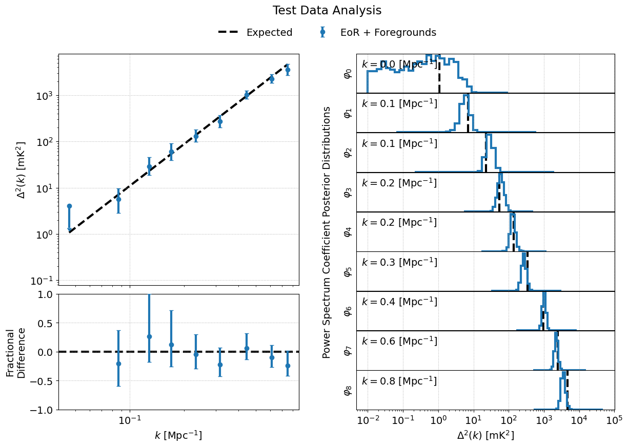
fig = data.plot_power_spectra_and_posteriors(
    suptitle="Test Data Analysis",
    plot_fracdiff=True,
    cred_interval=95,
    uplim_inds=uplim_inds
)

Note that, in the code block above, we added an additional kwarg, uplim_inds. For the provided EoR + foregrounds test dataset, the posterior in the lowest \(k\) bin produces a non-detection. For any non-detections, we can plot the upper limit, as the 95-th percentile, by using uplim_inds which acts like a mask. Any entries in uplim_inds which are True (False) will be plotted as an upper limit (detection: median plus credibility interval). uplim_inds must be a boolean numpy.ndarray with shape (len(dirnames), Nkbins) where Nkbins is the number of \(k\) bins in the analysis.

Attention

If you changed the location in which the sampler outputs are stored, you will need to update dir_prefix in the above code block to point to your specified output directory.

Tip

The bayeseor.analyze.analyze.DataContainer class calculates credibility intervals via the cred_intervals kwarg. You can specify any credibility intervals of interest as an e.g. list of percentages. By default, the 68% and 95% credibility intervals are calculated for each \(k\) bin. You can choose which credibility interval to plot as the uncertainty on each \(k\) bin in bayeseor.analyze.analyze.DataContainer.plot_power_spectra_and_posteriors() via the cred_interval kwarg.

This should produce the following figure if the analysis has been run correctly: