Running BayesEoR
run-analysis.py provides an example driver script for running BayesEoR. This file contains all of the necessary steps to set up the bayeseor.posterior.PowerSpectrumPosteriorProbability class and to run MultiNest and obtain power spectrum posteriors.
There are currently three steps involved in a BayesEoR analysis
Preprocess the data and generate an instrument model (uses only CPUs)
Build the required matrices (uses only CPUs, no GPUs required)
Run the power spectrum analysis (double precision GPUs required)
Below, we provide some useful information about the required Inputs and these Analysis Steps. For additional help with running BayesEoR and setting analysis parameters, please see Setting Parameters. More information on running BayesEoR can also be found below in Test Dataset.
Inputs
BayesEoR requires the following as inputs to run a power spectrum analysis:
Input data
Instrument model
A set of analysis and model parameters
More information about each of these components can be found below.
Input Data
The input dataset is expected to be a numpy-compatible, complex, one-dimensional vector of visibilities with shape (Nvis,). Here, Nvis = Nbls * Ntimes * Nfreqs is the total number of visibilities and Nbls, Ntimes, and Nfreqs is the number of baselines, times, and frequencies in the data. The ordering of the visibilities for each baseline, frequency, and time in this one-dimensional vector is arbitrary. However, this order must align with the ordering of the baselines in the instrument model (more on this below in Preprocessing the Data).
Instrument Model
The instrument model is comprised of several components
“uv sampling”: the specific (u, v, w) coordinates sampled by each baseline with shape (Ntimes, Nbls, 3)
Redundancy model: the number of baselines which sample each (u, v, w) coordinate in the uv sampling with shape (Ntimes, Nbls, 1)
Primary beam model: either a path to a UVBeam-compatible file or a string specifying an analytic beam profile (please see
bayeseor.model.healpix.Healpixfor details on supported analytic beam types and their associated parameters)Phasor vector (optional): an array which phases the visibilities as a function of time with shape (Nvis,)
Quantities 1-3 are required in every analysis. Quantity 4, the phasor vector, is optional and is only used if modelling phased visibilities. In our experience, we have found that we recover more accurate model visibilities when the data and model are unphased. For this reason, we suggest modelling unphased visibilities and excluding the phasor vector from the instrument model.
The uv sampling, redundancy model, and optional phasor vector can all be generated using the provided data preprocessing script scripts/data_preprocessing.py. Please see the section below on Preprocessing the Data for more information.
Choosing Analysis and Model Parameters
The example configuration file (example-config.yaml) provides an example of the minimum required analysis and model parameters which must be specified by the user for a power spectrum analysis. Please see Setting Parameters for the contents of this file and bayeseor.params.BayesEoRParser for a description of each of the user-definable analysis parameters. This information can also be displayed by running
python run-analysis.py --help
As stated in Setting Parameters, all of these parameters can be set via a configuration yaml file (recommended) or via the command line.
Some of these parameters have quite obvious values. For example, nf and nt are simply the number of frequencies and times in the data being analyzed, respectively. Other parameters require a little more care. The parameters nu (the number of sampled Fourier modes along the u axis of the model uv plane) and fov_ra_eor (the field of view of the sky model along the right ascension axis) must be chosen more carefully. In addition to the field of view of the sky model, fov_ra_eor also determines the spacing between adjacent modes along the u axis of the model uv plane. The value of nu must therefore be chosen to fully encompass the u coordinates sampled by the baseline in the input data. The beam must also be taken into account when choosing nu for a given fov_ra_eor as the beam effects the extent of the uv plane sampled by each baseline. The same arguments apply when choosing nv and fov_dec_eor as these quantities correspond to the v axis of the model uv plane and the declination axis of the sky model, respectively. Please see section 2.3 of Burba et al. 2023 for a more detailed discussion on choosing model parameters.
Analysis Steps
Preprocessing the Data
We have provided a script scripts/data_preprocessing.py which takes a pyuvdata-compatible file containing visibilities for each baseline, time, and frequency and generates the following numpy-compatible files
A one-dimensional visibility data vector
- An instrument model comprised of
uvw_model.npy: the “uv sampling” or (u, v) coordinates sampled by each baselineredundancy_model.npy: the redundancy of each baselinephasor_vector.npy(optional): a phasor vector which is used to phase the model visibilities as a function of time
It is also possible to store the instrument model as a python dictionary instead of separate files as indicated above. In the case of a dictionary, the uv sampling, redundancy model, and optional phasor vector must all be indexed by the keys 'uvw_model', 'redundancy_model', and 'phasor_vector', respectively. Please see bayeseor.model.instrument.load_inst_model for more details.
The provided data preprocessing script also uses jsonargparse for the command line interface. All of the command line arguments can thus be specified either via a configuration yaml file or via the command line directly. For a description of each of the command line arguments please see
python data_preprocessing.py --help
Note that this step is not required when running the test data (Test Dataset) as the test data have already been run through the preprocessing script.
Building the Matrix Stack
If using a configuration file (recommended), the driver script can be run to build the matrices via
python run-analysis.py --config /path/to/config.yaml --cpu
Note that with jsonargparse, command line arguments that come after the --config flag overwrite the value of the argument in the configuration file. In the example above, the --cpu flag placed after the --config flag will force the code to use CPUs only.
BayesEoR automatically creates a directory in which to store the matrix stack if one does not already exist. The name of the matrix stack directory is set automatically based on the chosen analysis parameters. The prefix for this matrix stack directory can be set via the array_dir_prefix argument in the configuration yaml or the --array-dir-prefix flag on the command line. The matrix stack is saved in a subdirectory within array_dir_prefix. The default matrix stack prefix is ./array-storage/.
Running the Power Spectrum Analysis
Once the matrices are built, you can run the power spectrum analysis (which requires double precision GPUs) via
python run-analysis.py --config /path/to/config.yaml --gpu
As above, the trailing --gpu flag will force the code to use GPUs. The power spectrum analysis will only run if at least one GPU is found and the GPU initialization is succesful.
Outputs
The location for the outputs of a BayesEoR analysis can be set via the output_dir argument in the configuration yaml or the --output-dir flag on the command line. The output files from BayesEoR will be placed in a subdirectory of output_dir and the name of the subdirectory is set automatically based on the chosen analysis parameters. The default output directory prefix is ./chains/.
BayesEoR outputs a few key files:
args.json: This file contains all of the configuration / command line arguments used for each analysis.k-vals*.txt: These files contain information about the spherically-averaged k bins.k-vals.txt: average magnitude of all k in each k bink-vals-bins.txt: bin edges of each k bink-vals-nsamples.txt: number of model k-cube voxels included in each k bin
data-*: These files contain the outputs of the sampler, the most important beingdata-.txt. This file contains the sampler output and has the power spectrum amplitude samples for each iteration. For MultiNest outputs, this file has Nkbins + 2 columns where Nkbins is the number of spherically-averaged k bins. The columns of interest in this file are the columns with index 0 and >= 2. The 0th column contains the joint posterior probability value per iteration. The columns with index >= 2 contain the power spectrum amplitude samples for each k bin.
For convenience, we have provided a class to aid in analyzing the aforementioned outputs of BayesEoR. For more information on this class, please see Analyzing BayesEoR Outputs.
Test Dataset
The BayesEoR repository provides a set of test data and an example yaml configuration file. The test data contain mock EoR only simulated visibilities with a Gaussian beam and a full width at half maximum of 9.3 degrees. For more information on the test data, see Section 3 of Burba et al. 2023.
To build the matrices (which will require ~17 GB of RAM and ~17 GB of disk space) using the provided example configuration yaml and test data, first navigate to the root directory of the BayesEoR repository and run
python run-analysis.py --config example-config.yaml --cpu
Note that, by default, the matrices will be stored in array-storage/ inside the BayesEoR repository. If you wish to change the location in which the matrices (or outputs) are stored, please see Setting Parameters. Once the matrices are built, you can run the power spectrum analysis (which will require ~12 GB of RAM) via
python run-analysis.py --config example-config.yaml --gpu
The mock EoR signal in the provided test data was generated as Gaussian white noise which has a flat power spectrum, P(k) = 214777.66068216303 mK^2 Mpc^3. BayesEoR outputs the dimensionless power spectrum which can be obtained from P(k) via e.g. Equation 13 Burba et al. 2023. The k bin values required to obtain the dimensionless power spectrum are written to disk automatically by BayesEoR in the same directory as the sampler outputs (please see Outputs or Analyzing BayesEoR Outputs for more information).
Analyzing BayesEoR Outputs
We have provided a basic class for analyzing the outputs of BayesEoR. The minimum requirement to instantiate the class is a list of directory names containing the BayesEoR output files. There are also several kwargs you can set to calculate various quantities, compare the results with an expected power spectrum, and/or modify the attributes of the created plots. Please see DataContainer Class Definition below for more information.
As an example, let us consider the case of analyzing the outputs of an analysis using the provided test data.
from pathlib import Path
from bayeseor.utils.analyze_results import DataContainer
dir_prefix = Path('./chains/')
dirnames = ['MN-Test-15-15-38-0-2-6.2E-03-2.63-2.82-lp-dPS-v1']
expected_ps = 214777.66068216303 # mK^2 Mpc^3
data = DataContainer(
dirnames, dir_prefix=dir_prefix, expected_ps=expected_ps, labels=['v1']
)
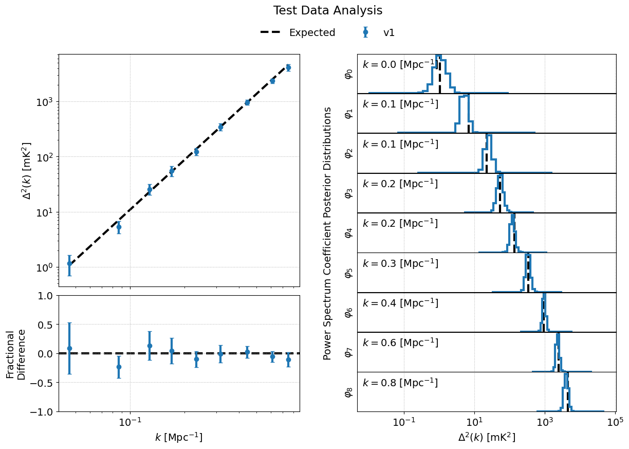
fig = data.plot_power_spectra_and_posteriors(
suptitle='Test Data Analysis', plot_fracdiff=True
)
In this example, we’ve assumed the default output location ./chains/. The subdirectory containing the BayesEoR output files is ./chains/MN-Test-15-15-38-0-2-6.2E-03-2.63-2.82-lp-dPS-v1/. Here, we are only analyzing the output from a single analysis. If you wish to compare multiple analyses within the same directory, i.e. you have multiple subdirectories containing output files in ./chains/, you can add more entries to dirnames e.g.
dirnames = ['MN-Test-15-15-38-0-2-6.2E-03-2.63-2.82-lp-dPS-v1',
            'MN-Test-15-15-38-0-2-6.2E-03-2.63-2.82-lp-dPS-v2',
            'MN-Test-15-15-38-0-2-6.2E-03-2.63-2.82-lp-dPS-v3']
The variable expected_ps in the example above has been set specifically for the test dataset. The mock EoR signal in the test dataset has a flat power spectrum, P(k) (more info in the section above on the Test Dataset). We thus only need to specify a floating point number for the expected P(k). The class will internally convert this P(k) into the dimensionless power spectrum, or vice versa, based on the combination of the ps_kind kwarg ('ps' for power spectrum or 'dmps' for the dimensionless power spectrum) and the expected_ps or expected_dmps kwargs. The default value of ps_kind is 'dmps', but we’ve passed the class the expected_ps kwarg corresponding to the power spectrum. The class will thus automatically convert this floating point P(k) into the corresponding dimensionless power spectrum using the k bins files in each output directory.
The DataContainer class also provides a few plotting functions. In the example above, we’re using the plot_power_spectra_and_posteriors function which creates a summary plot containing a subplot for the power spectrum estimates, an optional difference or fractional difference subplot if providing a known input power spectrum, and a subplot for the posterior of each k bin. This code snippet will produce the following output if the analysis has been run correctly:
DataContainer Class Definition
- class bayeseor.utils.analyze_results.DataContainer(dirnames, dir_prefix=None, sampler='multinest', calc_uplims=False, quantile=0.95, uplim_inds=None, Nhistbins=31, calc_kurtosis=False, ps_kind='dmps', temp_unit='mK', little_h_units=False, expected_ps=None, expected_dmps=None, labels=None)
Class for reading and analyzing files output by BayesEoR.
- Parameters:
dirnames (array-like of str) – Array-like of BayesEoR output directory names.
dir_prefix (str, optional) – Prefix to append to dirnames. Defaults to None, i.e. the entries in dirnames are assumed to be valid paths to BayesEoR output directories.
sampler (str, optional) – Case insensitive sampler name, e.g. ‘MultiNest’ or ‘multinest’ (default). The only currently supported sampler is MultiNest (default).
calc_uplims (bool, optional) – If calc_uplims is True, calculate the upper limit of each k bin’s posterior as the weighted 95th percentile using the joint posterior probability per iteration as the weights. Defaults to False.
quantile (float, optional) – Quantile in [0, 1]. Defaults to 0.95. Only used if calc_uplims is True.
uplim_inds (array-like, optional) – Array-like of True for non-detections and False for detections. Can have shape
(Nkbins,), whereNkbinsis the number of spherically averaged k bins with power spectrum posteriors in the sampler output or shape(len(dirnames), Nkbins). IfNkbinsvaries in each file, each entry in uplims must havelen(uplims[i]) == Nkbinsfor that particular file.Nhistbins (int, optional) – Number of histogram bins for each k bin’s posterior distribution.
calc_kurtosis (bool, optional) – If calc_kurtosis is True, calculate the kurtosis of each k bin’s posterior distribution.
ps_kind (str, optional) – Case insensitive power spectrum kind in the sampler output file. Can be ‘ps’ or ‘dmps’ for the power spectrum, P(k), or dimensionless power spectrum, Delta^2(k). Defaults to ‘dmps’.
temp_unit (str, optional) – Either ‘mK’ or ‘K’. The temperature unit of the power spectrum. The default output from BayesEoR is ‘mK’ (default).
little_h_units (bool, optional) – If little_h_units is True, power spectrum samples are assumed to be in units of little h. Defaults to False. Currently, BayesEoR picks the Planck 2018 value of the Hubble constant but we plan to output power spectra in little h units in the future. This kwarg has thus been added for future use.
expected_ps (float or array-like, optional) – Expected power spectrum, P(k). Can be a single float (for a flat P(k)) or an array-like with length equal to the number of spherically averaged k bins.
expected_dmps (float or array-like, optional) – Expected dimensionless power spectrum, Delta^2(k). Can be a single float or an array-like with length equal to the number of spherically averaged k bins.
labels (array-like of str, optional) – Array-like containing strings with shorthand labels for each directory in dirnames. Used in figure legends for plotting functions. Defaults to None (no labels).
- calculate_expected_ps(expected_ps=None, expected_dmps=None)
Calculated the expected power spectrum for each output file.
Sets either self.expected_ps if self.ps_kind is ‘ps’ or self.expected_dmps if self.ps_kind is ‘dmps’.
- Parameters:
expected_ps (float or array-like, optional) – Expected power spectrum, P(k). Can be a single float (for a flat P(k)) or an array-like with length equal to the number of spherically averaged k bins.
expected_dmps (float or array-like, optional) – Expected dimensionless power spectrum, Delta^2(k). Can be a single float or an array-like with length equal to the number of spherically averaged k bins.
- get_posterior_data(fp, Nkbins, q=0.95, Nhistbins=31, log_priors=True)
Load sampler output and form posteriors for each k bin.
- Parameters:
fp (str or Path) – Path to sampler output file.
Nkbins (int) – Number of spherically averaged k bins.
q (float, optional) – Quantile in [0, 1]. Defaults to 0.95. Only used if self.calc_uplims is True.
Nhistbins (int, optional) – Number of histogram bins for each k bin’s posterior distribution. Defaults to 31.
log_priors (bool, optional) – If log_priors is True (default), power spectrum samples are assumed to be in log10 units and are first linearized prior to calculating e.g. upper limits. Otherwise, the power spectrum samples are assumed to be in linear units.
- Returns:
posteriors (ndarray) – Posterior distributions for each k bin with shape
(Nkbins, Nhistbins)where Nkbins is the number of spherically averaged k bins in fp.avgs (ndarray) – Weighted average of each k bin posterior.
stddev (ndarray) – Weighted standard deviation of each k bin posterior.
uplims (ndarray (returned only if self.calc_uplims is True)) – q-th quantile of each k bin posterior.
kurtoses (ndarray (returned only if self.calc_kurtosis is True)) – Kurtosis of each k bin posterior.
- plot_posteriors(plot_height=1.0, plot_width=7.0, hspace=0, colors=None, cmap=None, lw=3, ls_expected='--', log_y=False, ymin=1e-16, show_k_vals=True, suptitle=None, fig=None, axs=None)
Plot power spectrum posteriors.
- Parameters:
plot_height (float, optional) – Subplot height. Defaults to 1.0.
plot_width (float, optioanl) – Subplot width. Defaults to 7.0.
hspace (float, optional) – matplotlib gridspec height space. Defaults to 0.05. Only used if plot_diff or plot_fracdiff is True.
colors (array-like of str, optional) – Array-like of valid matplotlib color strings. Must have length self.Ndirs. If None (default), use the default matplotlib color sequence.
cmap (callable matplotlib colormap instance, optional) – Callable matplotlib colormap instance, e.g. matplotlib.pyplot.cm.viridis. If None (default), use the default matplotlib color sequence.
lw (float, optional) – matplotlib line width. Defaults to 3.
ls_expected (str, optional) – Any valid matplotlib line style string. Used for plotting the expected power spectrum (used only if self.expected_ps or self.expected_dmps is not None). Defaults to ‘–‘.
log_y (bool, optional) – If log_y is True, plot the amplitudes of the posteriors in log10 units. Otherwise, plot the amplitudes of the posteriors in linear units (default).
ymin (float, optional) – Minimum value for the y axis. Used if log_y is True to avoid plotting very small y values. Defaults to 1e-16.
show_k_vals (bool, optional) – If show_k_vals is True (default), print the value of the k bin associated with each posterior in the upper left corner of each posterior subplot.
suptitle (str, optional) – Figure suptitle string. Defaults to None.
fig (Figure, optional) – matplotlib Figure instance. Used internally when called by self.plot_power_spectra_and_posteriors.
axs (Axes) – matplotlib Axes instance(s). Used internally when called by self.plot_power_spectra_and_posteriors.
- plot_power_spectra(uplim_inds=None, plot_height=4.0, plot_width=7.0, hspace=0.05, height_ratios=[1, 0.5], x_offset=0, zorder_offset=0, labels=None, colors=None, cmap=None, marker='o', capsize=3, lw=3, ls_expected='--', plot_diff=False, plot_fracdiff=False, ylim=None, ylim_diff=[-1, 1], legend_loc='best', legend_ncols=1, figlegend=False, top=0.85, suptitle=None, fig=None, axs=None)
Plot the power spectrum as the weighted average and std. dev.
- Parameters:
uplim_inds (array-like, optional) – Array-like of True for non-detections and False for detections. Can have shape
(Nkbins,), whereNkbinsis the number of spherically averaged k bins with power spectrum posteriors in the sampler output or shape(len(dirnames), Nkbins). IfNkbinsvaries in each file, each entry in uplims must havelen(uplims[i]) == Nkbinsfor that particular file. If uplim_inds is None (default), use self.uplim_inds. Otherwise, use uplim_inds in place of self.uplim_inds.plot_height (float, optional) – Subplot height. Defaults to 4.0.
plot_width (float, optioanl) – Subplot width. Defaults to 7.0.
hspace (float, optional) – matplotlib gridspec height space. Defaults to 0.05. Only used if plot_diff or plot_fracdiff is True.
height_ratios (array-like, optional) – matplotlib gridspec subplot height ratios. Defaults to [1, 0.5], i.e. the top plot will be twice as tall as the bottom subplot. Only used if plot_diff or plot_fracdiff is True.
x_offset (float, optional) – x-axis offset for plotting multiple results on a single subplot. If x_offset > 0, data points for different analyses will be offset along the x-axis to better distinguish overlapping data.
zorder_offset (int, optional) – matplotlib zorder offset for plotting multiple results on a single subplot. If zorder_offset > 0, data points for different analyses will be offset along the “z” axis (plot data points over or under each other).
labels (array-like of str, optional) – Array-like of label strings for each analysis result. If no labels are provided, checks for labels in self.labels. If self.labels is not None and labels is not None, the labels in labels will be used instead of self.labels. Must have length self.Ndirs. Defaults to None, i.e. use self.labels if not None otherwise use no labels.
colors (array-like of str, optional) – Array-like of valid matplotlib color strings. Must have length self.Ndirs. If None (default), use the default matplotlib color sequence.
cmap (callable matplotlib colormap instance, optional) – Callable matplotlib colormap instance, e.g. matplotlib.pyplot.cm.viridis. If None (default), use the default matplotlib color sequence.
marker (str, optional) – matplotlib marker string. Defaults to ‘o’.
capsize (float, optional) – Errorbar cap size. Defaults to 3.
lw (float, optional) – matplotlib line width. Defaults to 3.
ls_expected (str, optional) – Any valid matplotlib line style string. Used for plotting the expected power spectrum (used only if self.expected_ps or self.expected_dmps is not None). Defaults to ‘–‘.
plot_diff (bool, optional) – If plot_diff is True and self.expected_ps or self.expected_dmps is not None, plot the difference between each analysis’ power spectrum and the expected power spectrum. If both plot_diff and plot_fracdiff are True, plot_diff will be set to False and the fractional difference will be plotted instead. Defaults to False.
plot_fracdiff (bool, optional) – If plot_fracdiff is True and self.expected_ps or self.expected_dmps is not None, plot the fractional difference between each analysis’ power spectrum and the expected power spectrum. If both plot_diff and plot_fracdiff are True, plot_diff will be set to False and the fractional difference will be plotted instead. Defaults to False.
ylim (array-like, optional) – matplotlib ylim for the power spectrum subplot. Defaults to None (scales the y axis limits according to the data).
ylim_diff (array-like, optional) – matplotlib ylim for the (fractional) difference subplot if plot_diff or plot_fracdiff is True.
legend_loc (str, optional) – Any valid matplotlib legend locator string. Used only if figlegend is False. Defaults to ‘best’.
legend_ncols (int, optional) – Number of columns in the legend. Defaults to 1 unless figlegend is True. In the latter case, the default value is set to
self.Ndirs + 1.figlegend (bool, optional) – If figlegend is True, use a figure legend instead of an axes legend. Defaults to False.
top (float, optional) – Sets the top of the power spectrum subplot in figure fraction units (0, 1]. Defaults to 0.85.
suptitle (str, optional) – Figure suptitle string. Defaults to None.
fig (Figure, optional) – matplotlib Figure instance. Used internally when called by self.plot_power_spectra_and_posteriors.
axs (Axes) – matplotlib Axes instance(s). Used internally when called by self.plot_power_spectra_and_posteriors.
- plot_power_spectra_and_posteriors(uplim_inds=None, plot_height_ps=4.0, plot_width=7.0, hspace_ps=0.05, height_ratios_ps=[1, 0.5], x_offset=0, zorder_offset=0, labels=None, colors=None, cmap=None, marker='o', capsize=3, lw=3, ls_expected='--', plot_diff=False, plot_fracdiff=False, ylim_ps=None, ylim_diff_ps=[-1, 1], plot_height_post=1.0, hspace_post=0.01, log_y=False, ymin_post=1e-16, show_k_vals=True, legend_ncols=0, figlegend=True, top=0.875, right_ps=0.46, left_post=0.54, suptitle=None)
Make a plot containing power spectra and posteriors as subplots.
Calls self.plot_power_spectra and self.plot_posteriors.
- Parameters:
uplim_inds (array-like, optional) – Array-like of True for non-detections and False for detections. Can have shape
(Nkbins,), whereNkbinsis the number of spherically averaged k bins with power spectrum posteriors in the sampler output or shape(len(dirnames), Nkbins). IfNkbinsvaries in each file, each entry in uplims must havelen(uplims[i]) == Nkbinsfor that particular file. If uplim_inds is None (default), use self.uplim_inds. Otherwise, use uplim_inds in place of self.uplim_inds.plot_height_ps (float, optional) – Subplot height for the power spectra subplot(s). Defaults to 4.0.
plot_width (float, optioanl) – Subplot width for both the power spectra subplot(s) and the posterior subplots. Defaults to 7.0.
hspace_ps (float, optional) – matplotlib gridspec height space for the power spectra subplot(s). Defaults to 0.05. Only used if plot_diff or plot_fracdiff is True.
height_ratios_ps (array-like, optional) – matplotlib gridspec subplot height ratios for the power spectra subplots. Defaults to [1, 0.5], i.e. the top plot will be twice as tall as the bottom subplot. Only used if plot_diff or plot_fracdiff is True.
x_offset (float, optional) – x-axis offset for plotting multiple results on a single subplot. If x_offset > 0, data points for different analyses will be offset along the x-axis to better distinguish overlapping data.
zorder_offset (int, optional) – matplotlib zorder offset for plotting multiple results on a single subplot. If zorder_offset > 0, data points for different analyses will be offset along the “z” axis (plot data points over or under each other).
labels (array-like of str, optional) – Array-like of label strings for each analysis result. If no labels are provided, checks for labels in self.labels. If self.labels is not None and labels is not None, the labels in labels will be used instead of self.labels. Must have length self.Ndirs. Defaults to None, i.e. use self.labels if not None otherwise use no labels.
colors (array-like of str, optional) – Array-like of valid matplotlib color strings. Must have length self.Ndirs. If None (default), use the default matplotlib color sequence.
cmap (callable matplotlib colormap instance, optional) – Callable matplotlib colormap instance, e.g. matplotlib.pyplot.cm.viridis. If None (default), use the default matplotlib color sequence.
marker (str, optional) – matplotlib marker string. Defaults to ‘o’.
capsize (float, optional) – Errorbar cap size. Defaults to 3.
lw (float, optional) – matplotlib line width. Defaults to 3.
ls_expected (str, optional) – Any valid matplotlib line style string. Used for plotting the expected power spectrum (used only if self.expected_ps or self.expected_dmps is not None). Defaults to ‘–‘.
plot_diff (bool, optional) – If plot_diff is True and self.expected_ps or self.expected_dmps is not None, plot the difference between each analysis’ power spectrum and the expected power spectrum. If both plot_diff and plot_fracdiff are True, plot_diff will be set to False and the fractional difference will be plotted instead. Defaults to False.
plot_fracdiff (bool, optional) – If plot_fracdiff is True and self.expected_ps or self.expected_dmps is not None, plot the fractional difference between each analysis’ power spectrum and the expected power spectrum. If both plot_diff and plot_fracdiff are True, plot_diff will be set to False and the fractional difference will be plotted instead. Defaults to False.
ylim (array-like, optional) – matplotlib ylim for the power spectrum subplot. Defaults to None (scales the y axis limits according to the data).
ylim_diff (array-like, optional) – matplotlib ylim for the (fractional) difference power spectrum subplot if plot_diff or plot_fracdiff is True.
plot_height_post (float, optional) – Subplot height for the posterior subplots. Defaults to 1.0.
hspace_post (float, optional) – matplotlib gridspec height space for the posterior subplots. Defaults to 0.01.
log_y (bool, optional) – If log_y is True, plot the amplitudes of the posteriors in log10 units. Otherwise, plot the amplitudes of the posteriors in linear units (default).
ymin (float, optional) – Minimum value for the y axis of the posterior subplots. Used if log_y is True to avoid plotting very small y values. Defaults to 1e-16.
show_k_vals (bool, optional) – If show_k_vals is True (default), print the value of the k bin associated with each posterior in the upper left corner of each posterior subplot.
legend_ncols (int, optional) – Number of columns in the legend. Defaults to
self.Ndirs + 1.figlegend (bool, optional) – If figlegend is True (default), use a figure legend. Otherwise, no legend is shown.
top (float, optional) – Sets the top of the power spectrum and posterior subplots in figure fraction units (0, 1]. Defaults to 0.875.
right_ps (float, optional) – Sets the right edge of the power spectrum subplot(s) in figure fraction units (0, 1]. Defaults to 0.46.
left_post (float, optional) – Sets the left edge of the posterior subplot(s) in figure fraction units (0, 1]. Defaults to 0.54.
suptitle (str, optional) – Figure suptitle string. Defaults to None.